 1
 2
 3
 4
 5
 6
 7
 8
 9
10
11
12
13
14
15
16
17
18
19
20
21
22
23
24
25
26
27
28
29
30
31
32
33
34
35
36
37
38
39
40
41
42
43
44
45
46
47
48
49
50
51
52
53
54
55
56
57
58
59
60
61
62
63
64
65
66
67
68
69
70
71
72
73
74
75
76
77
78
|
import numpy as np
import matplotlib.pyplot as plt
# ==========================================
# 步骤 1: 模拟物理世界 (生成非线性数据)
# ==========================================
# 假设我们用 7 瓶标气做校准:0, 10, 20... 100 ppm
true_concentration = np.array([0, 10, 20, 40, 60, 80, 100])
# 模拟传感器的物理响应:
# V = 5 * (1 - e^(-0.015 * C))
# 这是一种典型的饱和响应,浓度越高,电压涨得越慢
A = 5.0 # 最大电压 (V)
k = 0.015
raw_voltage = A * (1 - np.exp(-k * true_concentration))
# 加一点点噪声,模拟真实电路的波动
np.random.seed(42)
raw_voltage += np.random.normal(0, 0.005, size=len(raw_voltage))
print("原始电压测量值 (V):", np.round(raw_voltage, 3))
# ==========================================
# 步骤 2: 算法核心 (计算线性化系数)
# ==========================================
# 目标:找到一个多项式 C = f(V),把电压 V 变回浓度 C
# 这里我们选用 3次多项式 (Cubic Fitting)
degree = 3
# polyfit(x, y, deg) -> 注意这里 x 是电压(输入), y 是浓度(目标)
coeffs = np.polyfit(raw_voltage, true_concentration, degree)
# 生成多项式函数对象
linearization_func = np.poly1d(coeffs)
print("\n--- 计算出的线性化系数 (存入单片机) ---")
print(f"a (3次项): {coeffs[0]:.4f}")
print(f"b (2次项): {coeffs[1]:.4f}")
print(f"c (1次项): {coeffs[2]:.4f}")
print(f"d (截距): {coeffs[3]:.4f}")
# ==========================================
# 步骤 3: 验证效果 (应用系数)
# ==========================================
# 把原始的弯曲电压带入公式,看看算出来的浓度是不是直的
calculated_concentration = linearization_func(raw_voltage)
print("\n校准后计算浓度 (ppm):", np.round(calculated_concentration, 1))
print("真实标准气浓度 (ppm):", true_concentration)
# ==========================================
# 步骤 4: 画图展示
# ==========================================
plt.figure(figsize=(12, 5))
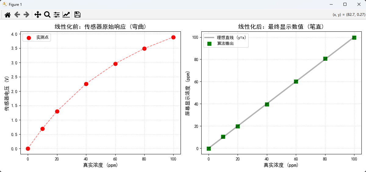
# 图1:拉直前(原始物理响应)
plt.subplot(1, 2, 1)
plt.scatter(true_concentration, raw_voltage, color='red', s=80, label='实测点')
plt.plot(true_concentration, raw_voltage, 'r--', alpha=0.5)
plt.title("线性化前:传感器原始响应 (弯曲)", fontsize=14)
plt.xlabel("真实浓度 (ppm)", fontsize=12)
plt.ylabel("传感器电压 (V)", fontsize=12)
plt.grid(True, linestyle=':', alpha=0.6)
plt.legend()
# 图2:拉直后(经过算法处理)
plt.subplot(1, 2, 2)
# 画出理想直线
plt.plot([0, 100], [0, 100], 'k-', alpha=0.3, linewidth=3, label='理想直线 (y=x)')
# 画出校准后的点
plt.scatter(true_concentration, calculated_concentration, color='green', marker='s', s=80, label='算法输出')
plt.title("线性化后:最终显示数值 (笔直)", fontsize=14)
plt.xlabel("真实浓度 (ppm)", fontsize=12)
plt.ylabel("屏幕显示浓度 (ppm)", fontsize=12)
plt.grid(True, linestyle=':', alpha=0.6)
plt.legend()
plt.tight_layout()
plt.show()
|